LEAP 71
PicoGK.org/coding for engineers
Thinking beyond Cartesian coordinates
We have been making good use of Cartesian coordinates in the past chapters, coordinates which are based on a system of three orthogonal axes, X, Y, and Z. We introduced the concept of a local coordinate system, represented by the Frame3d class, which allows us to orient the coordinate system independently of world coordinates. Using different Frame3d objects, we were able to place and orient parts to our hearts’ desires.
But while you always need three coordinates to represent a point in 3D space (and two for 2D space), there are other systems that are often better suited to a task. In this chapter, we will introduce Polar, Cylindrical, and Spherical coordinates, and how to use them in PicoGK.
One of the major advantages of choosing the right coordinate system is that the geometry often becomes dramatically simpler to describe algorithmically.
An apology
An apology first: many of you are familiar with these coordinate systems. So the following chapter may sound a bit repetitive, even trivial at times. You will, however, be using these systems a lot in Computational Engineering, so let’s over-explain, until you are so bored that you will not have to think about how they work ever again.
Polar coordinates
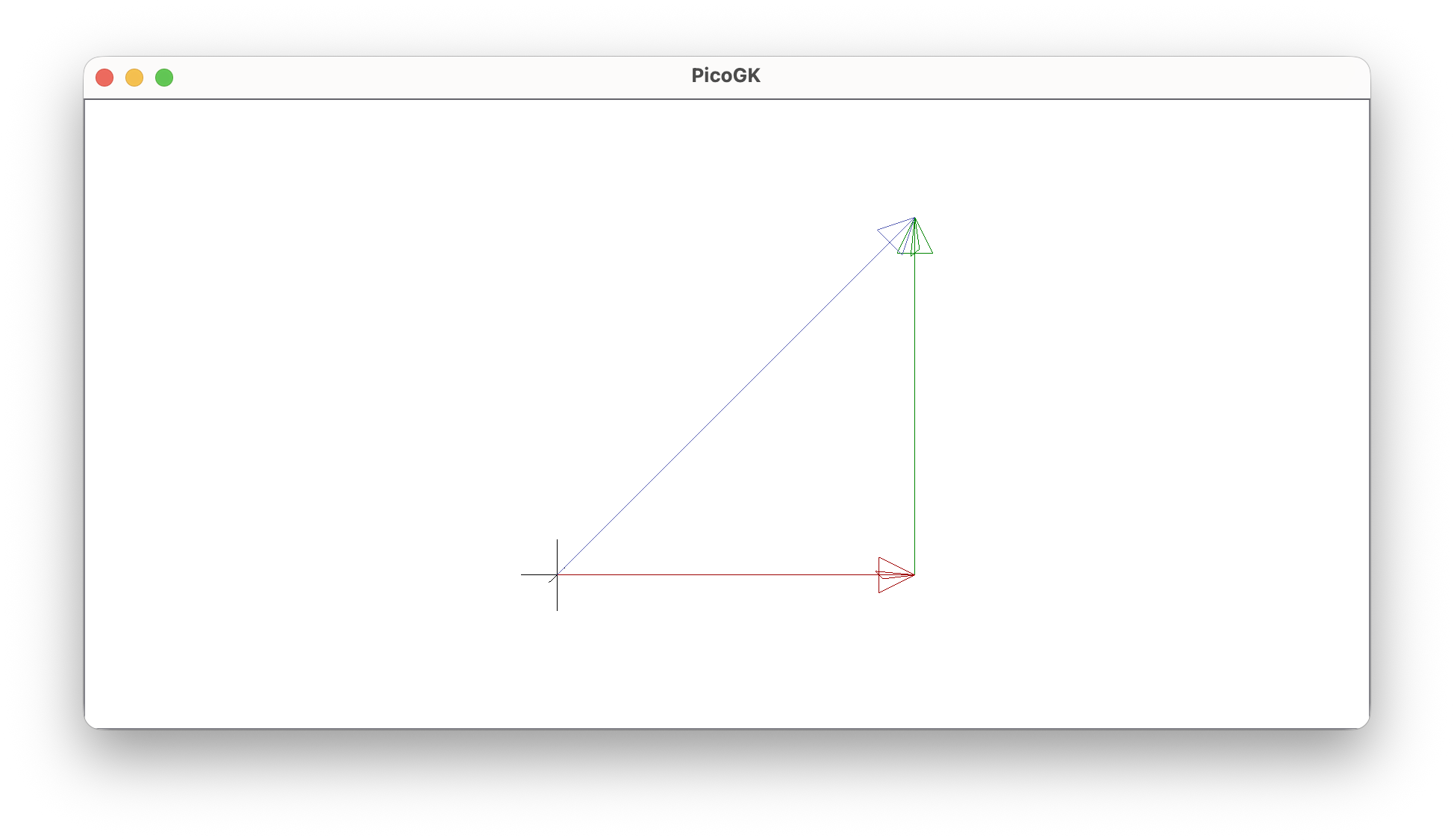
Let’s begin on a 2D plane and introduce the concept of Polar coordinates. On a flat 2D plane, we require two numbers to uniquely represent a point. In our standard Cartesian coordinate system, we use the Vector2 class, with its X and Y members. X and Y represent the distances along the respective axes from the origin, which lies at [0,0]. So a coordinate of X=1; Y=0; represents a point that lies 1 unit shifted in X and zero units shifted in Y.
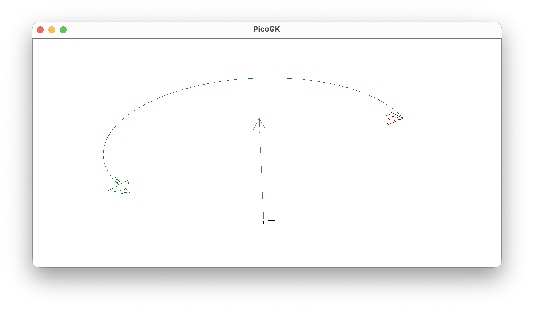
So, in the image below, the coordinate [1,1] (blue) is the result of moving 1 unit along the X axis (red), and 1 unit along the Y axis (green).
How else could you represent that point?
One way is to use Polar coordinates. We still have two dimensions, but one now represents the absolute distance of the point to the center of the coordinate system. What geometric shape consists of all points at the same distance from a reference point? A circle with radius R.
So let’s define a coordinate system with R, the radius, as one of the coordinates. What else do we need? An angle. If we specify the radius of a circle and the position on the circle using an angle, we have uniquely identified a point on a 2D plane.
While most people are used to specifying angles in degrees 0 to 360º, in mathematics, we specify angles using radians.
Radians are derived from the fact that the formula for the circumference of a circle is 2πr. For a circle with a radius of 1, you can simplify the circumference to 2π.
In other words, in math, an angle is actually the distance on a unit circle from 0 .. 2π, which in C# is 0 .. float.Pi * 2.
Since it’s cumbersome to constantly write float.Pi * 2, PicoGK defines a constant: Rad.TwoPi.
Where a full circle is float.Pi*2 (Rad.TwoPi), a half circle (180º) equals Rad.TwoPi/2, a quarter circle (90º) equals Rad.TwoPi/4. Etc. At first glance, the heavy use of Greek symbols may seem a little opaque, but radians are actually a remarkably intuitive system once you think about angles as distances along a circle. For completeness, one degree (1º) equals Rad.TwoPi/360.
So, radians it is. PicoGK has a Polar coordinate type, with two members, R and Phi. R is the distance of the point from the origin (the radius of the circle it is on). Phi is the angle, defining the position on that circle, in other words Phi is the azimuthal angle, the rotation around the central axis.
Here’s how it works:
Polar co = new();
co.R     = 10;
co.Phi   = Rad.TwoPi/4;
Since most of the time we are not working in Polar coordinates, the Polar type has a handy function to convert to Cartesian coordinates, which returns a Vector2:
Vector2 vecCartesian = co.vecAsCartesian();
So, let’s check this out in practice:
Polar coZero = new();
Vector2 vec2 = coZero.vecAsCartesian();
Vector3 vec3 = vec2.vecAsVector3();
Library.oViewer().AddCross(vec3);
We initialize a new Polar coordinate (coZero), convert it to Cartesian space, add a third dimension using vecAsVector3, and visualize the result with a cross in the viewer.
Just like with Vector2 and Vector3, Polar coordinates initialize to zero, in other words to the origin.
As expected, vec2 results in the coordinate [0,0] .
It’s probably a good idea at this point to highlight a curiosity of Polar coordinates: For the origin, with R equaling zero, Phi is undefined. Or more accurately, it doesn’t matter what number Phi has, if the distance R to the origin is zero, the point is (obviously) always at the origin. This is known as a coordinate singularity.
So let’s set our radius to something reasonable:
Polar co = new();
co.R = 1;
Console.WriteLine($"Polar={co} - Cartesian={co.vecAsCartesian()}");
Our coordinate now lies at a distance of 1 from the origin, at the angle Phi=0 (which is the default).
The above code shows us that a Polar coordinate of Radius=1; Phi=0; results in a Cartesian Vector2 of X=1; Y=0. So, we’ve established the direction of the angle, at position 0 it points towards the X axis of our orthogonal coordinate system. Let’s move Phi by a quarter circle (90º) in the positive direction and see where it points to:
co.Phi = Rad.TwoPi / 4;
Console.WriteLine($"Polar={co} - Cartesian={co.vecAsCartesian()}");
If you output this, you will get a weird number for X. This is expected and a common issue with floating point precision. Because π cannot be represented exactly in binary floating point, trigonometric functions often produce extremely small residual values instead of exact zeros.
Y on the other hand is clearly 1. So, by moving a quarter circle from Phi=0, (which translated to [1,0]), we now ended up at [0,1]. From this result, you can see the direction in which the coordinate system moves. PicoGK uses a right-handed coordinate system. Positive angular rotation is counter-clockwise when looking down the positive Z axis toward the origin. Our test just confirmed that.
If we move a half circle distance (180º), we will end up at [-1,0]:
co.Phi = Rad.TwoPi / 2;
Console.WriteLine($"Polar={co} - Cartesian={co.vecAsCartesian()}");
Again, you have to account for the floating point rounding issues, and ignore the tiny value you get for Y.
Let’s have some fun and plot the polar circle (sorry for the pun):
public static void PolarCircle()
{
    Polar coZero = new();

    Vector2 vec2 = coZero.vecAsCartesian();
    Vector3 vec3 = vec2.vecAsVector3();
    Library.oViewer().AddCross(vec3);

    Polar co = new();
    co.R = 10;

    int   nSteps = 20;
    float fStep  = Rad.TwoPi / nSteps;

    for (int n=0; n<nSteps;n++)
    {
        co.Phi = n * fStep;
        Library.oViewer().AddCross(co.vecAsCartesian().vecAsVector3());
    }
}
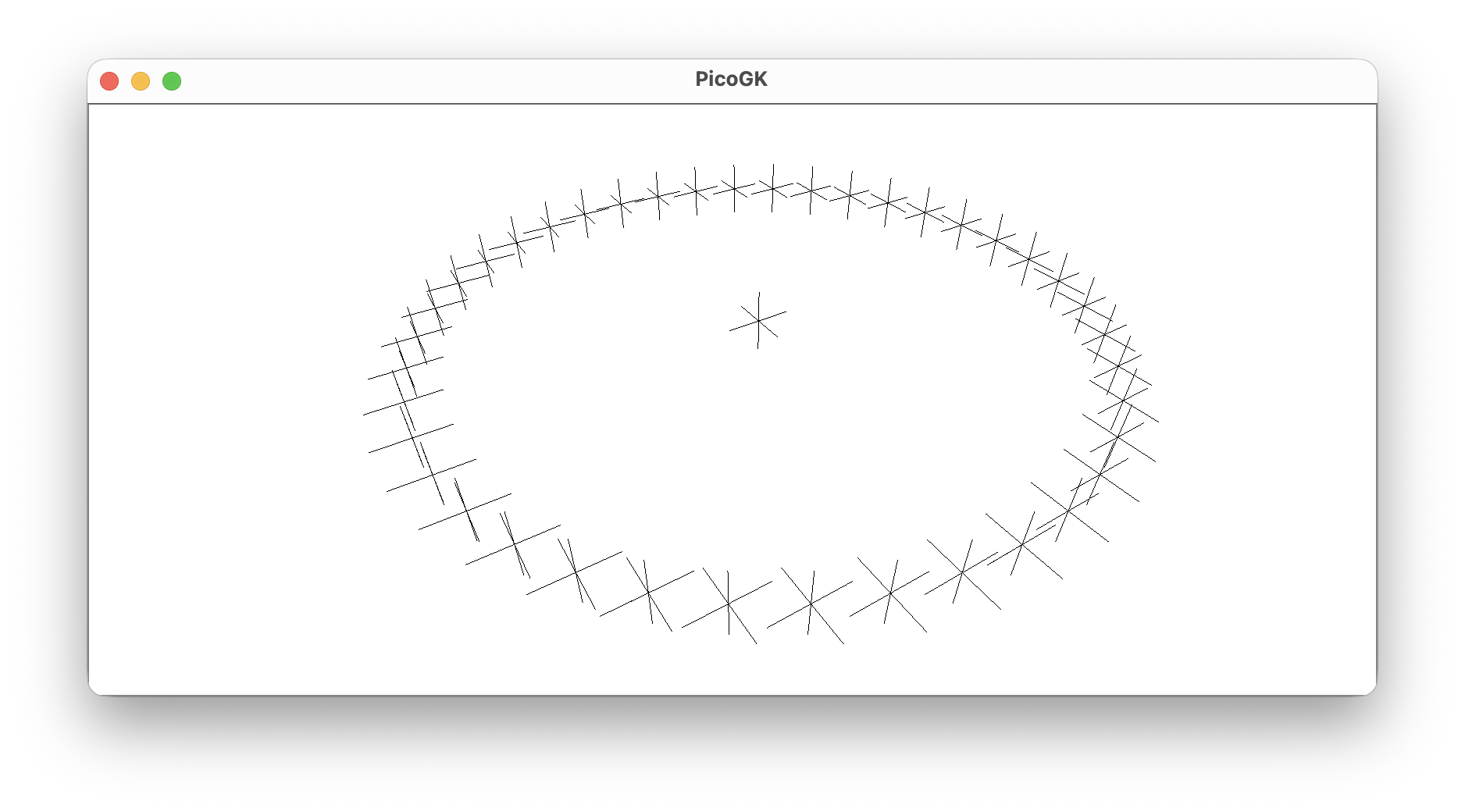
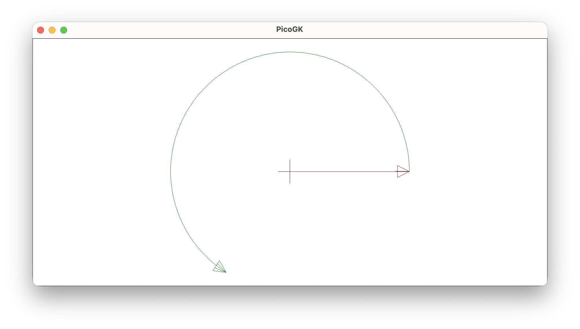
Let’s sum this up quickly. In Cartesian coordinates, we represent a point by specifying the distance from the origin for each orthogonal axis.
In Polar coordinates, a point is specified by the radius R (red) of the circle on which it lies, and the angle Phi (green) that determines the position on the circle.
Cylindrical coordinates
Polar coordinates are a good segue into a much more useful type of coordinate system. In fact, so useful, that we at LEAP 71 spend a lot of time, maybe most of our time there: If you look at many engineered objects, they are often rotationally symmetrical. Think of bolts, jet engines, pipes, what have you.
If you add a Z coordinate to a Polar coordinate, you end up with a Cylindrical coordinate, which specifies a point in 3D space.
Let’s rewrite our Polar example and just change the type:
public static void CylindricalCircle()
{
    Cylindrical coZero = new();
    Library.oViewer().AddCross(coZero.vecAsCartesian());

    Cylindrical co = new();
    co.R = 10;

    int     nSteps  = 20;
    float   fStep   = Rad.TwoPi / nSteps;

    for (int n=0; n<nSteps;n++)
    {
        co.Phi = n * fStep;
        Library.oViewer().AddCross(co.vecAsCartesian());
    }
}
As you can see, we no longer need the conversion to a Vector3, as vecAsCartesian already returns a 3D vector.
Well, to no one’s surprise, the example looks exactly like the PolarCircle example, as we didn’t do anything in Z.
Let’s move our point along the Z axis as we turn a full circle, and let’s draw an arrow from the center:
public static void CylindricalSpiral()
{
    Cylindrical coZero = new();
    Library.oViewer().AddCross(coZero.vecAsCartesian());

    Cylindrical co = new();
    co.R = 10;

    int     nSteps  = 40;
    float   fStep   = Rad.TwoPi / nSteps;
    float   fZStep  = 20f / nSteps;

    for (int n=0; n<nSteps;n++)
    {
        co.Phi      = n * fStep;
        coZero.Z    = n * fZStep;
        co.Z        = coZero.Z;

        Library.oViewer().AddArrow(coZero.vecAsCartesian(), co.vecAsCartesian());
    }
}
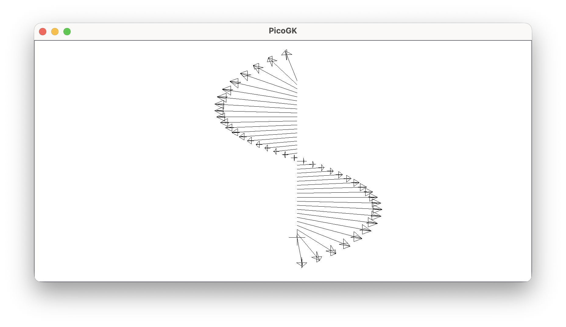
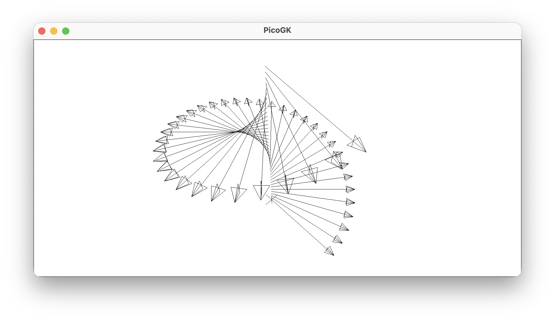
Now, that’s more 3D, isn’t it? You probably don’t need much imagination to consider what objects benefit from this type of coordinate system. Need to define the thread of a screw: Cylindrical coordinates. You need to place features around a rotationally symmetrical object? Cylindrical coordinates to the rescue.
Again, the simplest way to think about Cylindrical is Polar coordinates moved up (or down) the Z axis.
Spherical coordinates
What if we push the concept of angular coordinates even further? You end up with Spherical coordinates.
Where Cylindrical coordinates have Z, Spherical coordinates have another angle, Theta.
Note: Unfortunately, spherical coordinate conventions differ across mathematics, physics, CAD, and graphics systems. In PicoGK, Phi always represents the azimuthal angle around the Z axis (as with Polar and Cylindrical coordinates), while Theta represents the inclination from Z+ toward Z-.
The easiest way to think about Spherical coordinates is longitude and latitude on Earth, though mathematically Theta behaves more like an inclination measured from the North Pole. Latitude determines how far north or south you are, while longitude determines rotation around the Earth’s axis.
A Theta of 0 points straight up the Z+ axis. A Theta of Pi (half circle, 180º) points straight down to Z-.
A Theta of Pi/2 sits at the equator, halfway between the poles.
The radius R (red) again defines the distance of a point from the origin, but where R is the distance to the central axis of a cylinder in Cylindrical, in Spherical coordinates, R is the radial distance from the origin, defining a sphere. Just like with Polar and Cylindrical, a radius of 0 means that all coordinates map to the origin, regardless of the values of Phi (green) and Theta (blue).
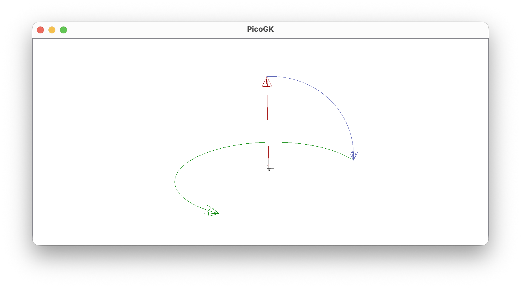
Just like at the North Pole and South Pole, longitude becomes degenerate at the poles: For a Theta of 0 (North Pole) and Pi (South Pole) all values of Phi map to the same point at the pole.
Below is the same value of Phi plotted at different values for Theta.
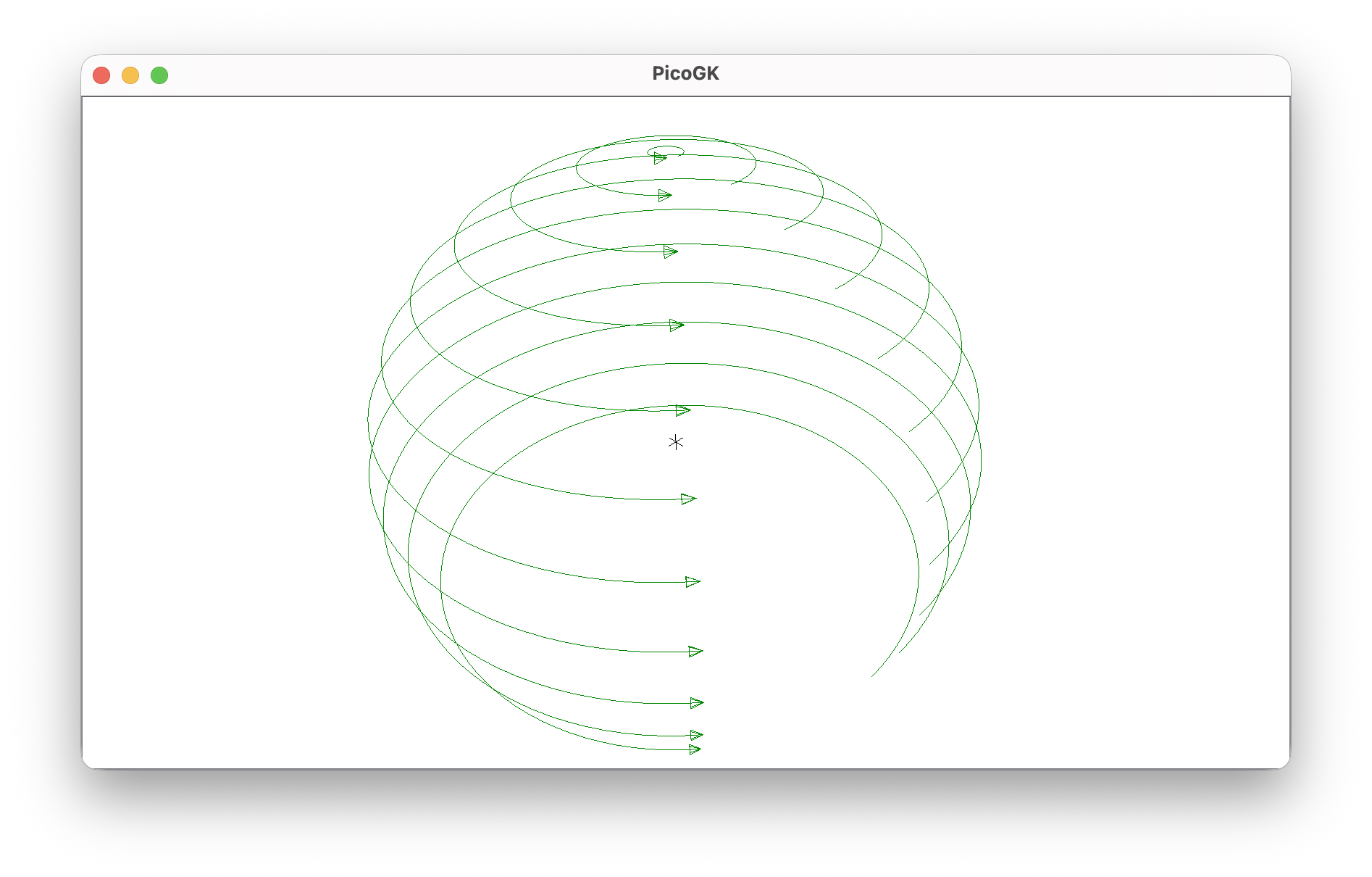
You can also see why we only need a half circle in Theta to reach every point on the surface of the sphere: Phi sweeps an entire circle for each value of Theta, so we can reach every point.
If you plot the same value of Theta for different values of Phi, it looks like this:
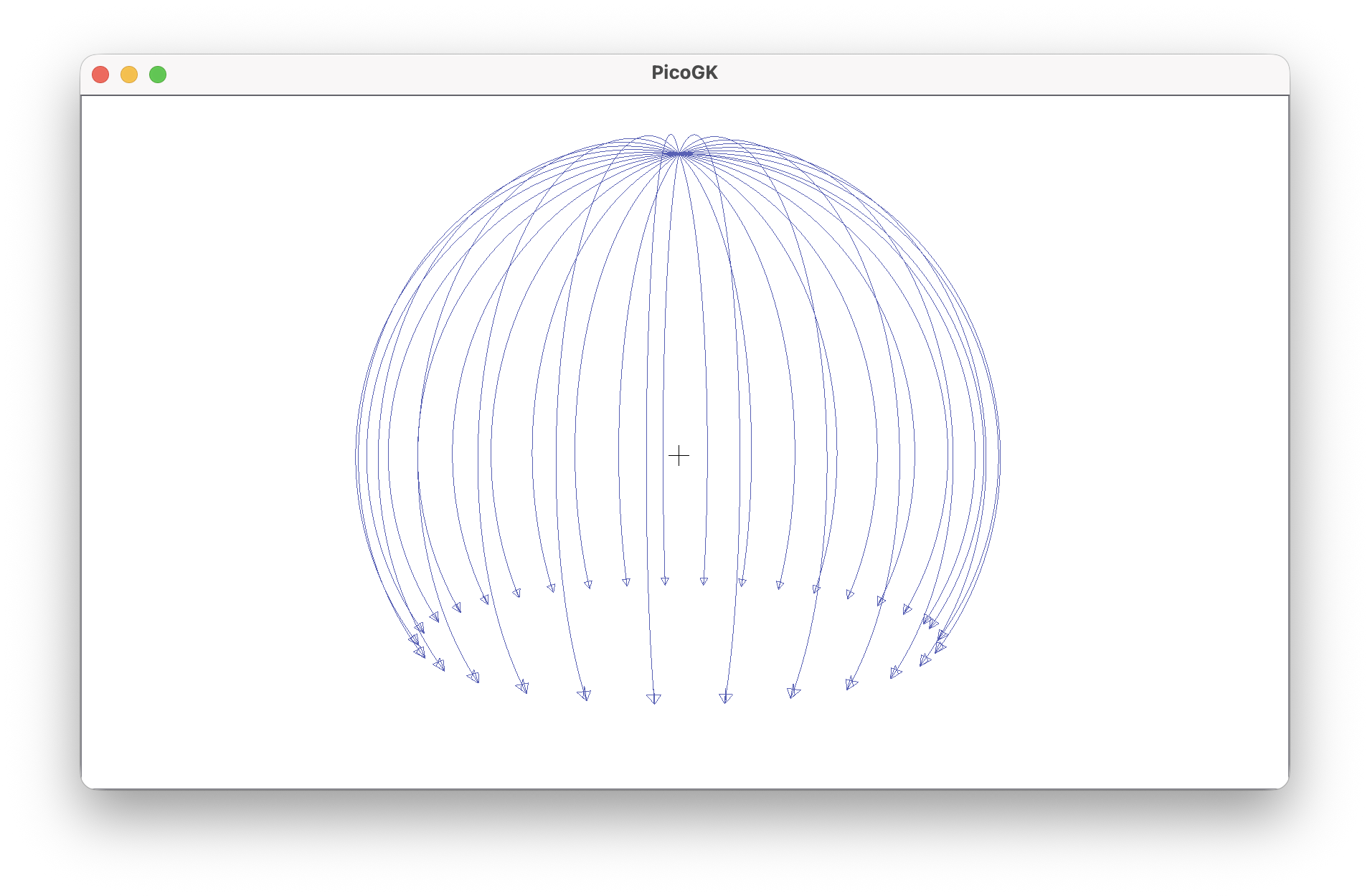
Let’s go through the following and let’s see if you can guess the output.
Spherical co = new();
co.R = 1;
Console.WriteLine($"Example 1: Spherical={co} - Cartesian={co.vecAsCartesian()}");

co.Theta = float.Pi / 2;
Console.WriteLine($"Example 2: Spherical={co} - Cartesian={co.vecAsCartesian()}");

co.Phi = Rad.TwoPi / 2;
Console.WriteLine($"Example 3: Spherical={co} - Cartesian={co.vecAsCartesian()}");

co.Theta = float.Pi;
Console.WriteLine($"Example 4: Spherical={co} - Cartesian={co.vecAsCartesian()}");
Let’s review:
- Example 1:
PhiandThetaare both zero. SinceThetais0, the coordinate lies at the North Pole regardless of the value ofPhi. The Cartesian vector is[0,0,1]. - Example 2:
Thetanow points halfway down the half circle, which means: to the equator. SincePhiis zero, the Cartesian coordinate now points along the positive X axis:[1,0,0](again ignoring floating point rounding). - Example 3: Now we set
Phito the value ofRad.TwoPi/2, which moves it half way around the globe. The Cartesian coordinate now points along the negativeXaxis:[-1,0,0]. - Example 4: We now set
ThetatoPi, which moves it to the South Pole: it now points straight down.Phihas no influence, since there’s only one position possible at the pole, since the diameter of the circle along whichPhimoves is zero:[0,0,-1].
Let’s place some objects
Enough with the lines and arrows. Let’s put these coordinates to use.
Let’s imagine we want to place objects in a circular manner.
public static void ObjectsAlongACircle()
{
    Polar co = new();

    co.R = 30;

    int   nSteps  = 10;
    float fStep   = Rad.TwoPi / nSteps;

    for (int n=0; n<nSteps; n++)
    {
        co.Phi = n * fStep;
        Vector3 vecPos = co.vecAsCartesian().vecAsVector3();
        Library.oViewer().Add(Voxels.voxSphere(vecPos, 2));
    }
}
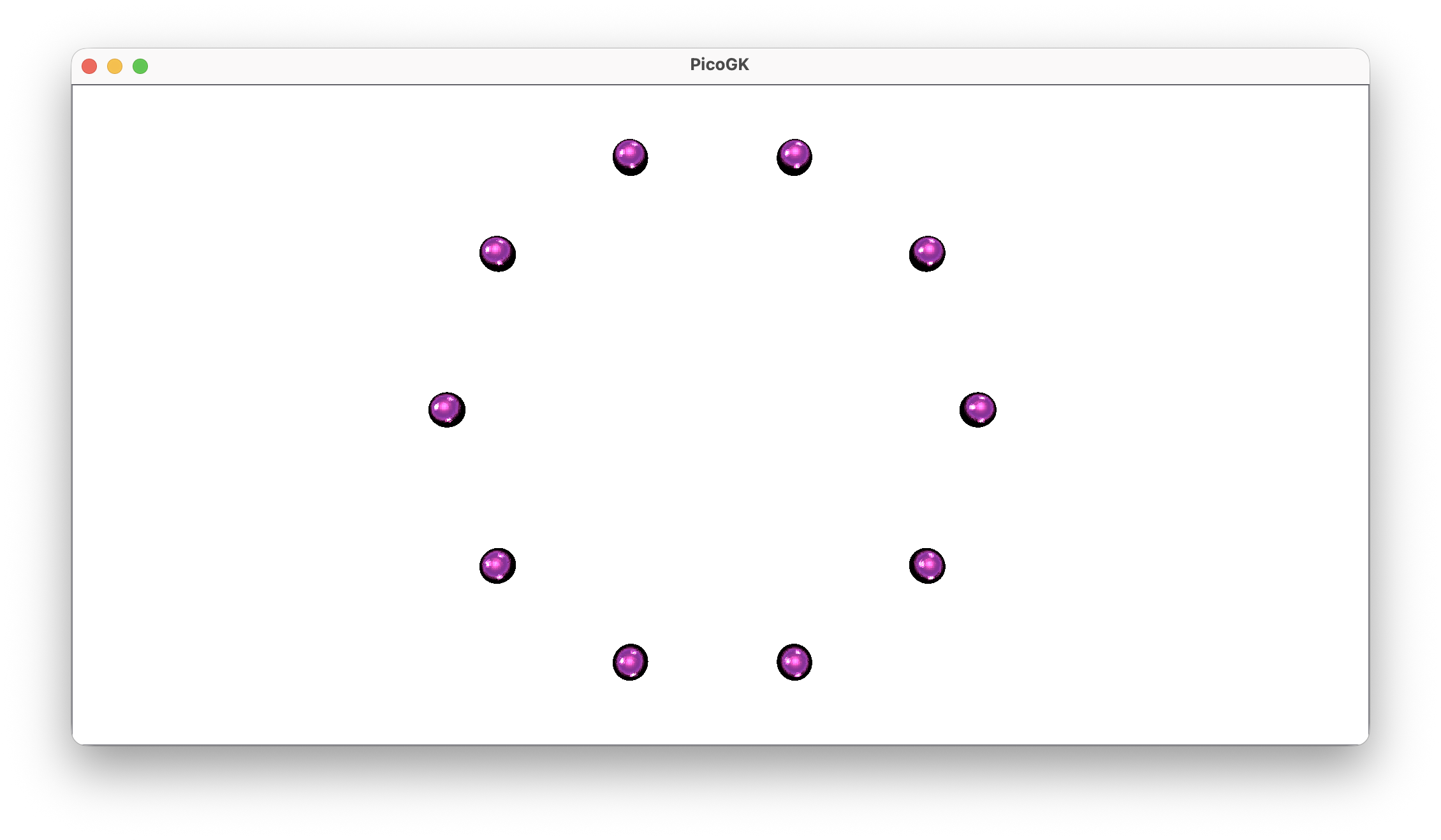
OK, nice, but not groundbreaking. What about some lattice beams that are actually aligned to face outwards?
Let’s modify the inner loop to create two coordinates:
co.Phi = n * fStep;
Vector3 vecPos = co.vecAsCartesian().vecAsVector3();

Polar coOuter = co;
coOuter.R += 10;
Vector3 vecOuter = coOuter.vecAsCartesian().vecAsVector3();

Library.oViewer().Add(Voxels.voxLatticeBeam(vecPos, 2, vecOuter, 1));
You can see, I could have gone about this in many different ways. I could have calculated the direction to the origin in Cartesian space, added that to the position, multiplied by a distance, for example.
But what I did instead is created a copy of the coordinate, increased the radius by 5 units, and used that as the tip of the object.
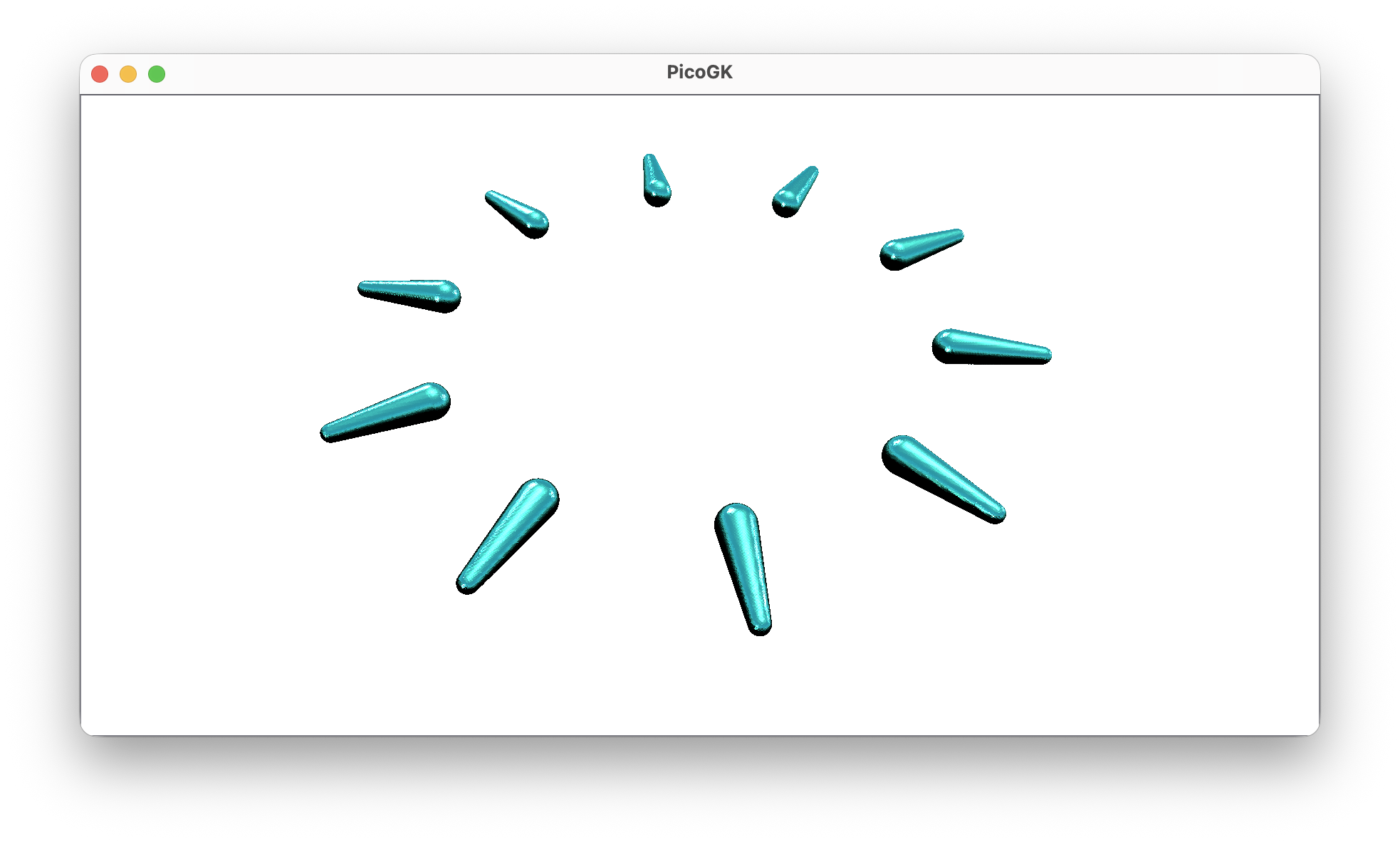
Let’s try the same in spherical coordinates:
Spherical co = new();
co.R = 20;

int nThetaSteps = 5;
float fThetaStep = float.Pi / (nThetaSteps-1);

int nPhiSteps = 10;
float fPhiStep = Rad.TwoPi / nPhiSteps;

for (int nTheta=0; nTheta<nThetaSteps; nTheta++)
{
    co.Theta = nTheta * fThetaStep;

    for (int nPhi=0; nPhi <nPhiSteps; nPhi++)
    {
        co.Phi          = nPhi * fPhiStep;
        Vector3 vecPos  = co.vecAsCartesian();

        Spherical coOuter = co;
        coOuter.R += 10;
        Vector3 vecOuter = coOuter.vecAsCartesian();

        Library.oViewer().Add(Voxels.voxLatticeBeam(vecPos, 1, vecOuter, .5f));
    }
}
Please note the subtle difference between the calculations of the steps for the Phi and Theta loops: While Phi needs to stop short of the full circle, to avoid placing two objects at the beginning and end of the circle (after 2*Pi we are back at position 0), for Theta we have to go the entire half circle, otherwise the object at the South Pole is missing, hence the float fThetaStep = float.Pi / (nThetaSteps-1); calculation, which ensures we include that coordinate.
Which gives us this result.
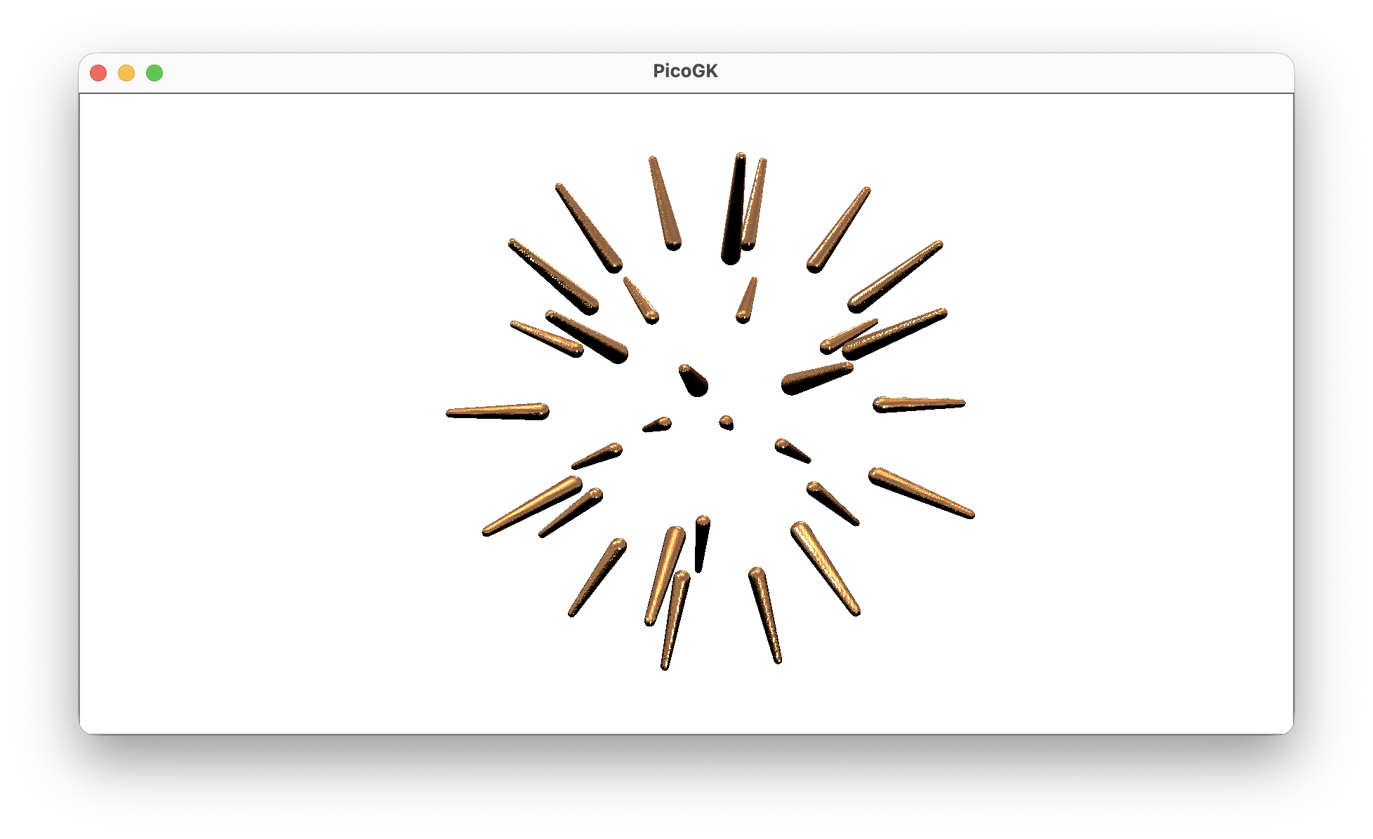
Great for a first demo. Now, there are a number of things we probably want to change: Because the longitudinal circles have smaller and smaller circumferences, the higher latitudes get pretty crowded with objects, as the distances decrease. At the poles the distance between the objects collapses to zero, resulting in many objects occupying exactly the same position. Probably not what we want.
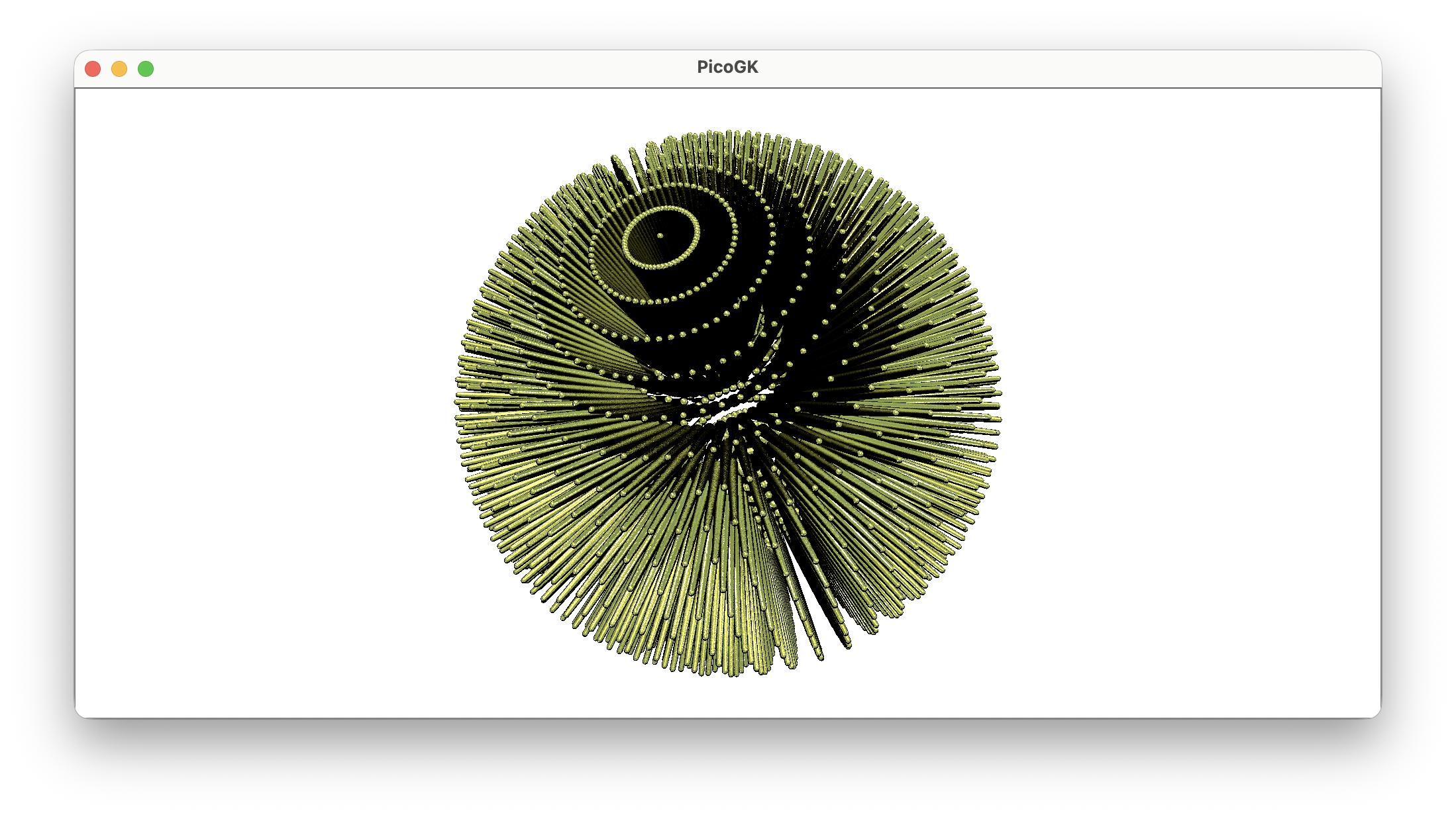
But we will leave this for the next chapter, where we will tie these coordinate systems to our Frame3d objects to start doing some more interesting things.
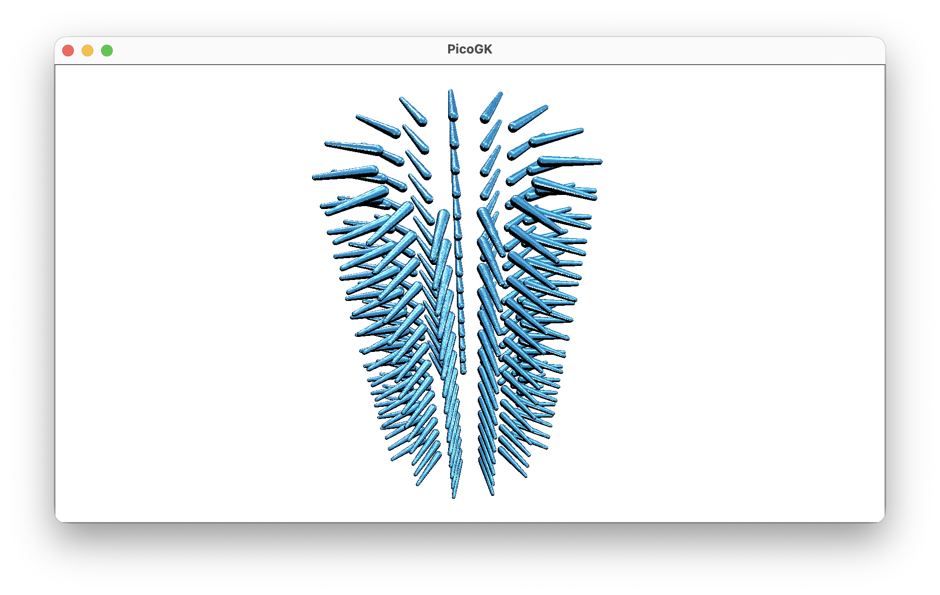
As a last step, since for cylinders, things are a little easier, let’s do the same exercise for a cylinder, and space our lattice beams evenly.
 Cylindrical co = new();
 co.R = 15;

 int nSteps = 15;
 float fPhiStep = Rad.TwoPi / nSteps;

 // Distance (on the circle), between each object: 2πR
 float fZStep = fPhiStep * co.R;

 for (int nZ=0; nZ<nSteps; nZ++)
 {
     co.Z = nZ * fZStep;

     for (int nPhi=0; nPhi <nSteps; nPhi++)
     {
         co.Phi          = nPhi * fPhiStep;
         Vector3 vecPos  = co.vecAsCartesian();

         Cylindrical coOuter = co;
         coOuter.R += 10;
         Vector3 vecOuter = coOuter.vecAsCartesian();

         Library.oViewer().Add(Voxels.voxLatticeBeam(vecPos, 1, vecOuter, .5f));
     }
 }
We take advantage of the fact that we can just multiply the fPhiStep with the radius to get the distance between the objects. We can use that as fZStep to evenly space the beams along the Z axis.
The other way around
Now, lastly, I should mention that of course you can also convert Cartesian coordinates to Polar, Cylindrical, and Spherical coordinates. This is less common than you might think, but of course it’s entirely supported.
Spherical coSph = new(Vector3.UnitX);
Console.WriteLine($"Spherical: {coSph}");
As you can see, you can just pass a Cartesian Vector3 (or Vector2 in the case of Polar) to the constructor and create a new corresponding coordinate.
If you plot the Phi values for different Cartesian coordinates, you will notice that the range is somewhat different than what we used in all our examples above. In this chapter, we continuously traveled along the circle (in counter-clockwise direction), increasing the value of Phi.
So for a Polar coordinate with an R of 1 the following table is true:
| Phi | Cartesian | ||
|---|---|---|---|
Rad.TwoPi * 0.00f |
0 |
[1,0] |
Positive X |
Rad.TwoPi * 0.25f |
π*0.5 |
[0,1] |
Positive Y |
Rad.TwoPi * 0.50f |
π |
[-1,0] |
Negative X |
Rad.TwoPi * 0.75f |
π*1.5 |
[0,-1] |
Negative Y |
We increase Phi by a quarter distance of the full circle (0.25f) at each step, and the coordinate moves counter-clockwise around the circumference.
But of course you can also travel the other way around, decreasing the value of Phi, which is just as valid:
| Phi | Cartesian | ||
|---|---|---|---|
Rad.TwoPi * -0.00f |
0 |
[1,0] |
Positive X |
Rad.TwoPi * -0.25f |
-π*0.5 |
[0,-1] |
Negative Y |
Rad.TwoPi * -0.50f |
-π |
[-1,0] |
Negative X |
Rad.TwoPi * -0.75f |
-π*1.5 |
[0,1] |
Positive Y |
A value of -float.Pi and a value of float.Pi points to the same position, halfway around the circle.
When you convert from Cartesian coordinates, Phi ends up in a range of -float.Pi .. +float.Pi and not 0 .. 2*float.Pi as you might have expected.
Here’s how this looks like in practice. In a way it’s intuitive that negative Cartesian coordinates also produce negative values of Phi.
| Cartesian | Phi | ||
|---|---|---|---|
[1,0] |
Positive X | Rad.TwoPi * 0.00 |
0 |
[0,1] |
Positive Y | Rad.TwoPi * 0.25 |
π*0.5 |
[-1,0] |
Negative X | -Rad.TwoPi * 0.50 |
-π |
[0,-1] |
Negative Y | -Rad.TwoPi * 0.25 |
-π*0.5 |
Just something to be aware of, when converting from Cartesian coordinates. The math stays the same, the range is still 2π — it doesn’t really matter where you start and in which direction you travel. A Phi of 0 continues to always point to the positive X direction.
Summary
As a Computational Engineer, you will spend a lot of time working in different coordinate systems. Traditional CAD systems, derived from the concept of a drafting table, tend to keep you thinking in Cartesian sketches, extrusions, and orthogonal feature operations, even when the underlying geometry is fundamentally radial or rotational.
But many engineered objects — turbines, pipes, pressure vessels, nozzles, bolts, threads, lattices — are far more naturally described using Cylindrical or Spherical coordinates.
In this chapter you:
- learned about
Polar,Cylindrical, andSphericalcoordinates - understood why angles in mathematics are measured in radians
- learned to think about angles as distances along a unit circle
- started placing geometry intuitively in non-Cartesian coordinate systems
As always, the code for this chapter is on GitHub
Next: Strong typing — An angle is not just a float
PicoGK.org/coding for engineers
© 2024-2026 by Lin Kayser — All rights reserved.